Data Analysis
Let’s take a look at what the data from the flight computer looks like. This data was recorded by an Arduino, logging telemetry once per second from the GPS and various sensors sensors and recorded them once a second. More details and the source code of the flight computer can be located at https://github.com/sea7aero/horizon2.
from preamble import *
%matplotlib inline
plt.rcParams['figure.figsize'] = (16, 5)
plt.rcParams['figure.dpi']= 150

directory = '../data'

# The flight tracker records invalid values as "*", so we want to replace those with Not a Number (NaN).
data = pd.read_csv(directory + '/raw-data.csv', na_values="*")
data.head()
| millis | year | month | day | hour | minute | second | voltage | satellites | hdop | gps_altitude_m | course | speed_mps | latitude | longitude | temperature_C | pressure_Pa | pressure_altitude_m | humidity_RH | Unnamed: 19 | |
|---|---|---|---|---|---|---|---|---|---|---|---|---|---|---|---|---|---|---|---|---|
| 0 | 1544 | NaN | NaN | NaN | NaN | NaN | NaN | 4.40 | NaN | NaN | NaN | NaN | NaN | NaN | NaN | 19.31 | 93891.82 | 638.10 | 42.74 | NaN |
| 1 | 2546 | 2000.0 | 0.0 | 0.0 | 0.0 | 0.0 | 0.0 | 4.37 | 0.0 | 99.99 | NaN | NaN | NaN | NaN | NaN | 19.36 | 93894.09 | 637.90 | 43.11 | NaN |
| 2 | 3547 | 2000.0 | 0.0 | 0.0 | 0.0 | 0.0 | 0.0 | 4.40 | 0.0 | 99.99 | NaN | NaN | NaN | NaN | NaN | 19.38 | 93892.00 | 638.09 | 42.69 | NaN |
| 3 | 4550 | 2000.0 | 0.0 | 0.0 | 0.0 | 0.0 | 0.0 | 4.40 | 0.0 | 99.99 | NaN | NaN | NaN | NaN | NaN | 19.39 | 93899.64 | 637.41 | 42.37 | NaN |
| 4 | 5551 | 2000.0 | 0.0 | 0.0 | 0.0 | 0.0 | 0.0 | 4.40 | 0.0 | 99.99 | NaN | NaN | NaN | NaN | NaN | 19.41 | 93896.39 | 637.70 | 42.41 | NaN |
Clean up the data
The raw data is a bit noisy - especially the first dozen seconds or so before the GPS acquired its lock - so the first step is to clean up the invalid data and a few other transformations in order to make it easier to work with.
# The tracker stores each part of the timestamp in a different column. To make it easier for us to work with and
# graph, we convert those columns into a single timestamp column, and make it the index of the Pandas dataframe.
datetime_cols = ["year", "month", "day", "hour", "minute", "second"]
timestamps = data[datetime_cols].apply(lambda x: "{:.0f}-{:.0f}-{:.0f} {:.0f}:{:.0f}:{:.0f}".format(*x), axis=1)
data["timestamp"] = pd.to_datetime(timestamps, errors="coerce")
data.drop(datetime_cols, axis=1)

# The first few rows don't have a valid timestamp at all; we'll just get rid of them.
data = data[data["timestamp"].notnull()]
data.index = data["timestamp"]
data = data.drop(["timestamp"], axis=1)

# # Fill any missing data with the last known value.  Then backfill missing data at the beginning of the file.
data = data.ffill().bfill()

# # Removes the extraneous "unnamed" column.
data = data.dropna(how="all", axis=1)

data.head()
| millis | year | month | day | hour | minute | second | voltage | satellites | hdop | gps_altitude_m | course | speed_mps | latitude | longitude | temperature_C | pressure_Pa | pressure_altitude_m | humidity_RH | |
|---|---|---|---|---|---|---|---|---|---|---|---|---|---|---|---|---|---|---|---|
| timestamp | |||||||||||||||||||
| 2021-09-25 17:26:17 | 21594 | 2021.0 | 9.0 | 25.0 | 17.0 | 26.0 | 17.0 | 4.40 | 0.0 | 99.99 | 656.1 | 0.0 | 0.1 | 47.160809 | -120.84832 | 19.56 | 93893.46 | 637.96 | 42.33 |
| 2021-09-25 17:26:18 | 22598 | 2021.0 | 9.0 | 25.0 | 17.0 | 26.0 | 18.0 | 4.40 | 0.0 | 99.99 | 656.1 | 0.0 | 0.1 | 47.160809 | -120.84832 | 19.56 | 93896.89 | 637.65 | 42.08 |
| 2021-09-25 17:26:19 | 23600 | 2021.0 | 9.0 | 25.0 | 17.0 | 26.0 | 19.0 | 4.37 | 0.0 | 99.99 | 656.1 | 0.0 | 0.1 | 47.160809 | -120.84832 | 19.58 | 93898.86 | 637.48 | 41.96 |
| 2021-09-25 17:26:20 | 24604 | 2021.0 | 9.0 | 25.0 | 17.0 | 26.0 | 20.0 | 4.40 | 0.0 | 99.99 | 656.1 | 0.0 | 0.1 | 47.160809 | -120.84832 | 19.59 | 93894.25 | 637.89 | 42.06 |
| 2021-09-25 17:26:21 | 25607 | 2021.0 | 9.0 | 25.0 | 17.0 | 26.0 | 21.0 | 4.40 | 0.0 | 99.99 | 656.1 | 0.0 | 0.1 | 47.160809 | -120.84832 | 19.59 | 93891.08 | 638.17 | 42.25 |
That’s much better, but we turned the tracker on before launch, and that data is kind of boring, so let us compute some interesting time spans and crop our data to just the mission data.
# Figure out the launch time by when it starts ascending.
ascent_rate = data['gps_altitude_m'].diff()
launch_index = np.argmax(ascent_rate > 3)
launch_millis = data['millis'][launch_index]
launch_time = data.index[launch_index]
data['mission_millis'] = data['millis'] - launch_millis

burst_index = np.argmax(data['gps_altitude_m'])
burst_time = data.index[burst_index]

# Figure out the landing time by when it stopped descending.
landing_index = len(ascent_rate) - np.argmax(ascent_rate.iloc[::-1] < -3)
landing_millis = data['millis'][launch_index]
landing_time = data.index[landing_index] # TODO: Determine this value, it may not be the last data.

print("Launch Time (UTC) : {}".format(launch_time))
print("Burst Time        : {}".format(burst_time))
print("Landing Time      : {}".format(landing_time))

ascent_duration = burst_time - launch_time
descent_duration = landing_time - burst_time
mission_duration = ascent_duration + descent_duration

print("Mission Duration  : {}".format(mission_duration))
print("Ascent Duration   : {}".format(ascent_duration))
print("Descent Duration  : {}".format(descent_duration))
Launch Time (UTC) : 2021-09-25 17:28:11
Burst Time        : 2021-09-25 20:04:25
Landing Time      : 2021-09-25 20:41:37
Mission Duration  : 0 days 03:13:26
Ascent Duration   : 0 days 02:36:14
Descent Duration  : 0 days 00:37:12
mission_data = data[launch_index:landing_index].copy()
mission_data.tail()
| millis | year | month | day | hour | minute | second | voltage | satellites | hdop | gps_altitude_m | course | speed_mps | latitude | longitude | temperature_C | pressure_Pa | pressure_altitude_m | humidity_RH | mission_millis | |
|---|---|---|---|---|---|---|---|---|---|---|---|---|---|---|---|---|---|---|---|---|
| timestamp | ||||||||||||||||||||
| 2021-09-25 20:41:33 | 11728210 | 2021.0 | 9.0 | 25.0 | 20.0 | 41.0 | 33.0 | 4.37 | 12.0 | 0.73 | 364.4 | 34.4 | 4.8 | 47.188889 | -119.438377 | 23.58 | 96866.77 | 377.97 | 31.80 | 11593195 |
| 2021-09-25 20:41:34 | 11729211 | 2021.0 | 9.0 | 25.0 | 20.0 | 41.0 | 34.0 | 4.37 | 12.0 | 0.79 | 358.9 | 51.6 | 3.2 | 47.188900 | -119.438339 | 23.63 | 96920.57 | 373.33 | 31.76 | 11594196 |
| 2021-09-25 20:41:35 | 11730215 | 2021.0 | 9.0 | 25.0 | 20.0 | 41.0 | 35.0 | 4.37 | 12.0 | 0.79 | 353.4 | 76.4 | 2.6 | 47.188892 | -119.438301 | 23.68 | 96992.07 | 367.16 | 31.70 | 11595200 |
| 2021-09-25 20:41:36 | 11731216 | 2021.0 | 9.0 | 25.0 | 20.0 | 41.0 | 36.0 | 4.37 | 12.0 | 0.90 | 348.0 | 97.6 | 3.0 | 47.188877 | -119.438271 | 23.73 | 97054.25 | 361.80 | 31.62 | 11596201 |
| 2021-09-25 20:41:37 | 11732219 | 2021.0 | 9.0 | 25.0 | 20.0 | 41.0 | 37.0 | 4.37 | 12.0 | 0.75 | 342.9 | 112.1 | 3.5 | 47.188862 | -119.438232 | 23.77 | 97115.67 | 356.50 | 31.64 | 11597204 |
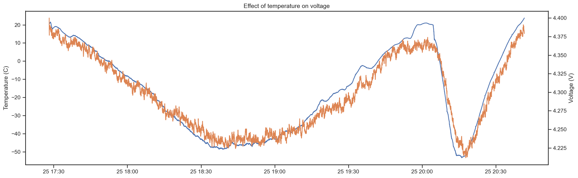
Camera Shutoff
In Graupel-1, we had a failure of the GoPro camera at around the Tropopause. We determined this was due to the 16850 battery we were using to charge the GoPro getting cold, reducing its output voltage, and causing a shut off.
For Graupel-2, we used a large, commercial external battery bank to power both the GoPro and the flight computer. We insulated the battery with some foam and added a hand warmer for good measure.
It looks like it worked well to keep the battery above critical voltages:
ax = pretty_plots()
ax.plot(mission_data['temperature_C'])
ax2 = ax.twinx()
ax2.plot(mission_data['voltage'].ewm(span=30).mean(), color='C1')
ax.set_title("Effect of temperature on voltage")
ax.set_ylabel("Temperature (C)")
ax2.set_ylabel("Voltage (V)")

print(f"Minimum temperature {mission_data['temperature_C'].min()}C")
print(f"Minimum voltage {mission_data['voltage'].min()}V")
Minimum temperature -53.3C
Minimum voltage 4.13V
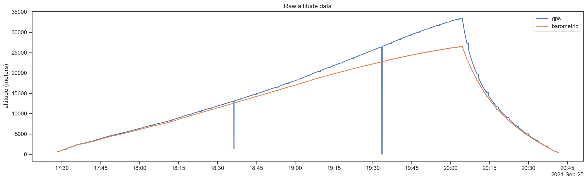
Altitude
The next thing to look at is the altitude, of course. In our case, we have 2 sources of data for the altitude: the value reported by the GPS and a value derived from the barometric pressure sensor. Let’s see what we’ve got…
ax = pretty_plots()
ax.plot(mission_data[["gps_altitude_m", "pressure_altitude_m"]])
ax.set_ylabel("altitude (meters)")
ax.legend(["gps", "barometric"])
ax.set_title('Raw altitude data')

difference = (mission_data["gps_altitude_m"] - mission_data["pressure_altitude_m"]).max()
print(f"Maximum altitude discrepency: {difference:.0f} meters")
Maximum altitude discrepency: 7005 meters
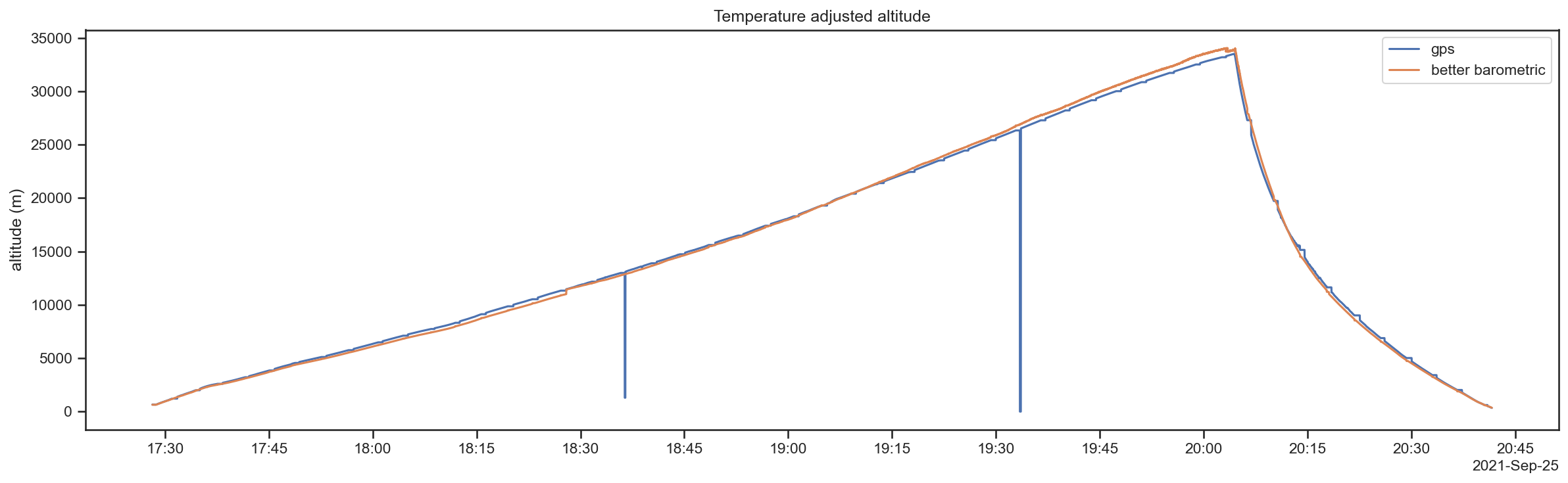
Correcting the barometric altitude
From Graupel-1, we learned that the tracker computes altitude from the barometric pressue using a naive algorithm that assumes you are in the Troposphere, which is the cause of the variation betweent he two readings. Let’s go ahead and apply what we learned there to this data.
# Here, we're loading up the ISA atmopsheric conditions and defining some constants.
isa = pd.read_csv(directory + '/standard-atmosphere.csv', index_col="layer").sort_values('base_pressure_Pa')

def annotate_layers(ax, label=True, max_layer=10):
    for index, layer in isa.iterrows():
        if(index < max_layer):
            altitude=layer['geopotential_altitude_m']
            ax.axhline(altitude, color='black', ls='-.', lw=0.25)
            if(label):
                ax.text(0.01, altitude+400, layer['name'], transform=ax.get_yaxis_transform())

display(isa)
| name | geopotential_altitude_m | geometric_altitude_m | lapse_rate_K_m | base_temperature_C | base_temperature_K | base_pressure_Pa | base_density_kg_m3 | |
|---|---|---|---|---|---|---|---|---|
| layer | ||||||||
| 7 | Mesopause | 84852 | 86000 | NaN | -86.28 | 186.87 | 0.37 | NaN |
| 6 | Mesosphere | 71000 | 71802 | -0.0020 | -58.50 | 214.65 | 3.96 | NaN |
| 5 | Mesosphere | 51000 | 51413 | -0.0028 | -2.50 | 270.65 | 66.94 | NaN |
| 4 | Stratopause | 47000 | 47350 | 0.0000 | -2.50 | 270.65 | 110.91 | 0.0020 |
| 3 | Stratosphere | 32000 | 32162 | 0.0028 | -44.50 | 228.65 | 868.02 | 0.0132 |
| 2 | Stratosphere | 20000 | 20063 | 0.0010 | -56.50 | 216.65 | 5474.90 | 0.0880 |
| 1 | Tropopause | 11000 | 11019 | 0.0000 | -56.50 | 216.65 | 22632.00 | 0.3639 |
| 0 | Troposphere | -610 | -611 | -0.0065 | 19.00 | 292.15 | 108900.00 | 1.2985 |
universal_gas_constant = 8.31432 # R, N*m/mol*K
molar_mass_dry_air = 0.0289644 # M, kg/mol
gas_constant_dry_air = universal_gas_constant / molar_mass_dry_air
gravitational_acceleration = 9.80665 # g0, m/s^2
# R / g0 * M
altitude_constants = -1.0 * gas_constant_dry_air / gravitational_acceleration

def calc_altitude(pressure):
    layer = isa['base_pressure_Pa'].searchsorted(pressure)
    parameters = isa.iloc[layer]
    base_altitude = parameters['geopotential_altitude_m']
    base_temperature = parameters['base_temperature_K']
    pressure_ratio = pressure / parameters['base_pressure_Pa']
    lapse_rate = parameters['lapse_rate_K_m']

    if lapse_rate == 0:
        factor = altitude_constants * base_temperature
        return base_altitude + factor * math.log(pressure_ratio)
    else:
        factor = base_temperature / lapse_rate
        exponent = altitude_constants * lapse_rate
        return base_altitude + factor * (pow(pressure_ratio, exponent)-1)

calc_altitude = np.vectorize(calc_altitude)
# From: https://commons.erau.edu/cgi/viewcontent.cgi?article=1124&context=ijaaa
def calc_altitude_temp_adjusted(pressure_Pa, temperature_C):
    temperature_K = temperature_C + 273.15
    layer = isa['base_pressure_Pa'].searchsorted(pressure_Pa)
    parameters = isa.iloc[layer]

    base_altitude_m = parameters['geopotential_altitude_m']
    base_temperature_K = parameters['base_temperature_K']
    temp_ratio = base_temperature_K / temperature_K

    pressure_ratio = pressure_Pa / parameters['base_pressure_Pa']

    density_ratio = pressure_ratio * temp_ratio
    lapse_rate = parameters['lapse_rate_K_m']

    if lapse_rate == 0:
        factor = altitude_constants * base_temperature_K
        return base_altitude_m + factor * math.log(density_ratio)
    else:
        factor = base_temperature_K / lapse_rate
        exponent = altitude_constants * lapse_rate
        return base_altitude_m + factor * (pow(density_ratio, exponent)-1)

calc_altitude_temp_adjusted = np.vectorize(calc_altitude_temp_adjusted)
def calc_altitude_blended(pressure_Pa, temperature_C):
    if(pressure_Pa > 22632):
        return calc_altitude(pressure_Pa)
    else:
        return calc_altitude_temp_adjusted(pressure_Pa, temperature_C)

calc_altitude_blended = np.vectorize(calc_altitude_blended)
mission_data['blended_altitude_m'] = calc_altitude_blended(mission_data['pressure_Pa'], mission_data['temperature_C'])
ax = pretty_plots()
ax.plot(mission_data[['gps_altitude_m', 'blended_altitude_m']])
ax.set_ylabel("altitude (m)")
ax.legend(["gps", "better barometric"]);
ax.set_title("Temperature adjusted altitude")

difference = mission_data["gps_altitude_m"] - mission_data["blended_altitude_m"]
print(f"Maximum altitude discrepency: {difference.max():.0f} meters")
Maximum altitude discrepency: 1046 meters
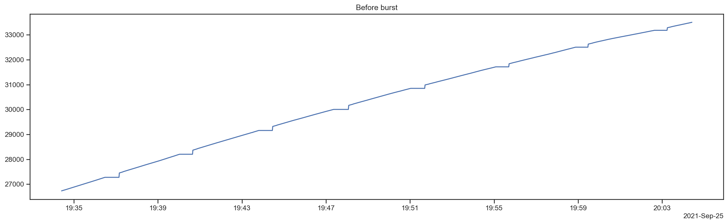
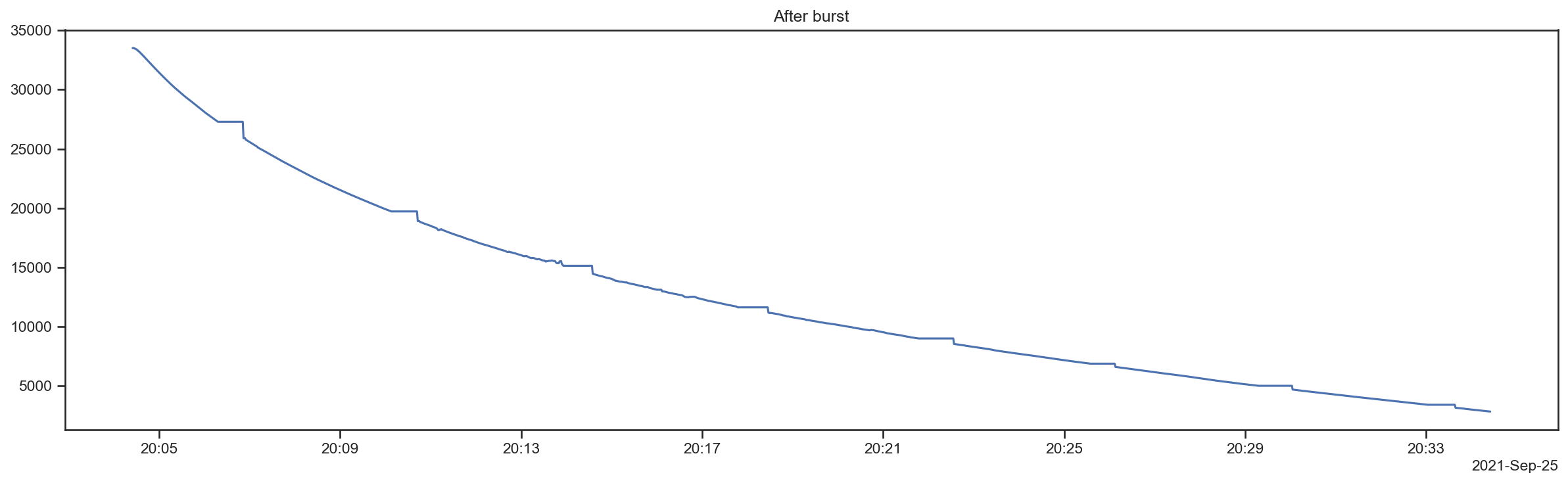
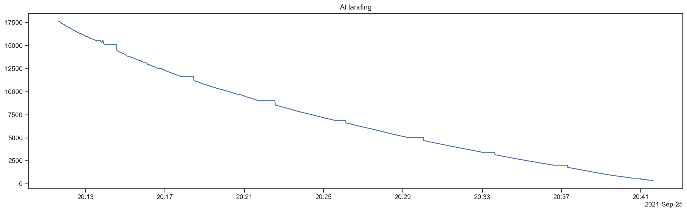
GPS altitude noise
Okay, now the barometric altitude looks better, but what about those weird jags in the GPS data? Those were not there in the Graupel-1 launch. Let’s take a closer look.
import datetime
window = datetime.timedelta(minutes=30)

def plot_window(title, start, end):
    fig, ax = plt.subplots(tight_layout=True)

    locator = mdates.MinuteLocator(byminute=range(60), interval=4)
    formatter = mdates.ConciseDateFormatter(locator)
    ax.xaxis.set_major_locator(locator)
    ax.xaxis.set_major_formatter(formatter)

    ax.plot(data[start:end]['gps_altitude_m'])
    ax.set_title(title)

plot_window('At launch', launch_time, launch_time + window)
plot_window('Before burst', burst_time - window, burst_time)
plot_window('After burst', burst_time, burst_time + window)
plot_window('At landing', landing_time - window, landing_time)
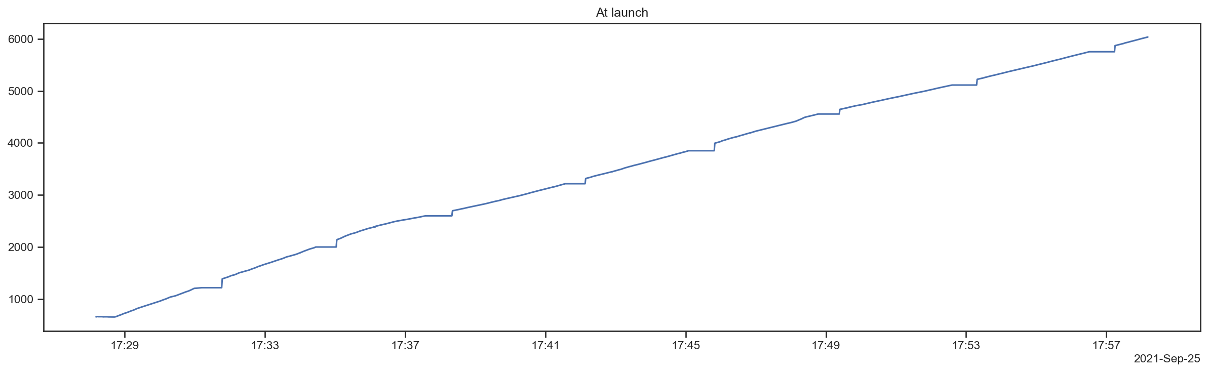
Smoothing noise
The noise in the GPS altitude is still a mystery to me. It seems that roughly every 4 minutes, through the entire flight, the GPS fails to update its altitude. It does not appear to be correlated to any other data as far as I can tell. If anyone has an idea, I’d love to hear it.
However, we can correct the data fairly well.
The first thing we can do is simply discard the obvious outliers where the GPS data was dropped using a “hampel” filter.
from hampel import hampel

filtered_altitude = hampel(mission_data['gps_altitude_m'], window_size=10, n=3, imputation=True)
ax = pretty_plots()

ax.plot(mission_data['gps_altitude_m'], label="unfiltered")
ax.plot(filtered_altitude, label="filtered")
ax.legend();
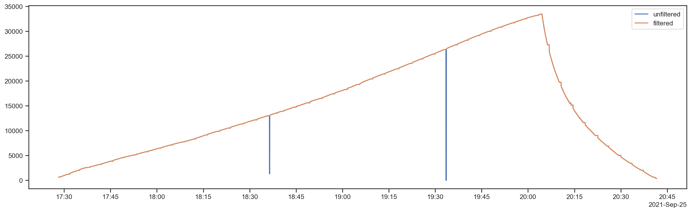
Next we can detect the discrepencies pretty easily by noting that the difference between one data point and the next is exactly 0. This happens rather rarely in real data, so we can simply throw those data points out and interpolate to fill the gaps.
# Replaces data points where the differences is 0 with NaN.
reject_noise = filtered_altitude.where(filtered_altitude.diff() != 0)

# Fill those NaNs through linear interpolation.
mission_data['altitude_m'] = reject_noise.interpolate()


ax = pretty_plots()
ax.set_title('Smoothed altitude')
ax.plot(mission_data['altitude_m'], label='altitude')
ax.set_ylabel('altitude (m)')

ax2 = ax.twinx()
ax2.plot(mission_data['altitude_m'].diff(), color='C1');
ax2.set_ylabel('ascent rate (m/s)')
Text(0, 0.5, 'ascent rate (m/s)')
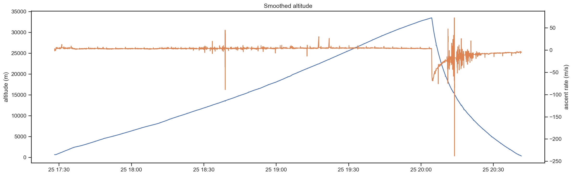
Alright, that looks pretty reasonable, though with some fairly rough nosie during a portion of the descent phase.
Altitude statistics
Finally, we can now compute some interesting altitude statistics and use them to answer some questions about our mission.
burst_altitude_index = np.argmax(mission_data['altitude_m'])
burst_altitude_m = mission_data['altitude_m'].max() * units.m
burst_altitude_ft = burst_altitude_m.to(units.ft)

print(f"Burst altitude: {burst_altitude_m.magnitude:0.1f} meters, ({burst_altitude_ft.magnitude:0.1f} feet)")
Burst altitude: 33502.8 meters, (109917.3 feet)
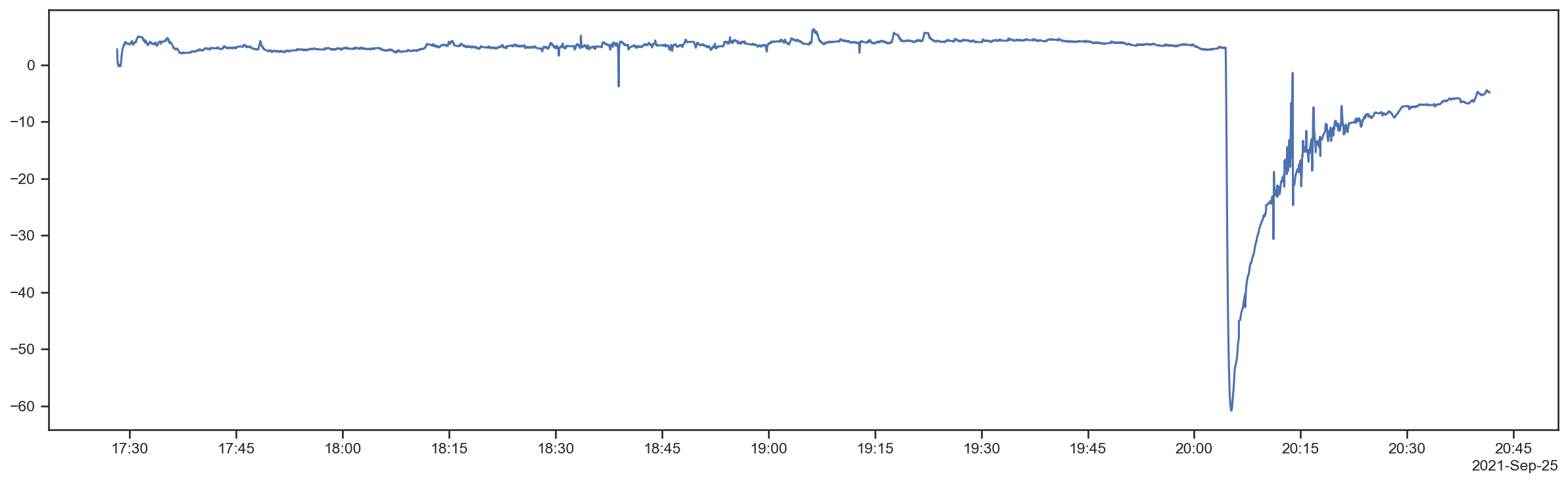
# We can smooth out a bit of the noise in the ascent rate data with a simple exponential moving average.
ascent_rate = mission_data['altitude_m'].diff()
mission_data['ascent_rate_mps'] = ascent_rate.ewm(span=30).mean()

ax = pretty_plots()
ax.plot(mission_data['ascent_rate_mps'])

ascent_phase = mission_data[mission_data.index < burst_time].copy()
descent_phase = mission_data[mission_data.index > burst_time].copy()

print("Maximum ascent rate: {0:0.2f} m/s".format(ascent_phase['ascent_rate_mps'].max()))
print("Average ascent rate: {0:0.2f} m/s".format(ascent_phase['ascent_rate_mps'].mean()))
print()
print("Maximum descent rate: {0:0.2f} m/s".format(descent_phase['ascent_rate_mps'].min()*-1))
print("Average descent rate: {0:0.2f} m/s".format(descent_phase['ascent_rate_mps'].mean()*-1))
print("Ascent rate at landing: {0:0.2f} m/s".format(descent_phase['ascent_rate_mps'][-1]*-1))
Maximum ascent rate: 6.36 m/s
Average ascent rate: 3.53 m/s

Maximum descent rate: 60.84 m/s
Average descent rate: 14.91 m/s
Ascent rate at landing: 4.87 m/s
Other Fun Data
Horizontal speed
In Graupel-1, our balloon reached horizontal speeds of up to 90 mph. This time, our balloon strolled along a more leisurely pace. This is good, because our ascent rate was lower than anticipated… if it was any faster, we would have had to drive to Idaho.
mission_data['speed_mps'] = mission_data['speed_mps'].ewm(alpha=0.05).mean()

fig, ax = plt.subplots()
annotate_layers(ax, label=True, max_layer=4)

ax.plot(mission_data['speed_mps'], mission_data['altitude_m'])
#ax.plot(descent_phase['speed_mps'], descent_phase['altitude_m'])

ax.set_title("Speed at altitude")
ax.set_xlabel("speed (m/s)")
ax.set_ylabel("altitude (meters)")

mph = units.mile / units.hour
max_speed = mission_data['speed_mps'].max() * units.m / units.s
print(f"Max speed: {max_speed.to(mph):0.2f}")
Max speed: 97.55 mile / hour
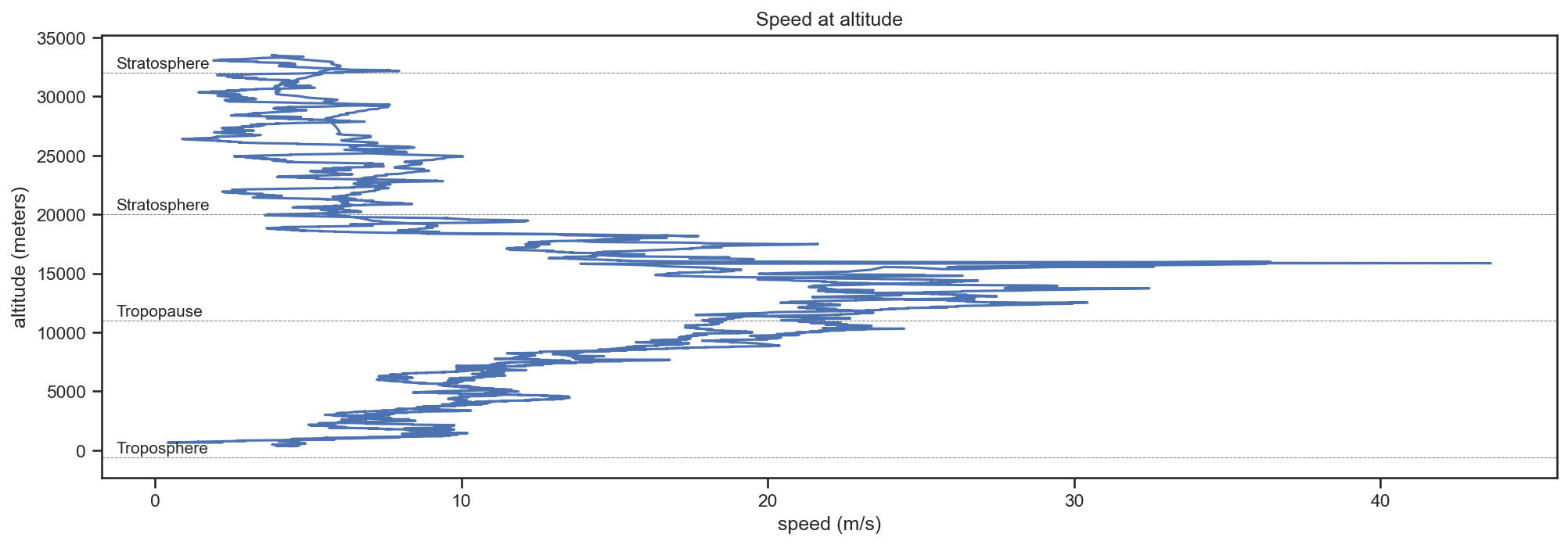
From the above data, we can see why our balloon travelled so far east from its predicted flight path. Our original estimated ascent rate was 4.9 m/s, but since we ran out of helium before hitting our target lift, our actual ascent rate averaged only 3.9 m/s. This caused our balloon to drift through the jet stream for a longer period of time, where it was being blown around at a brisk 35 m/s (~80 mph)!
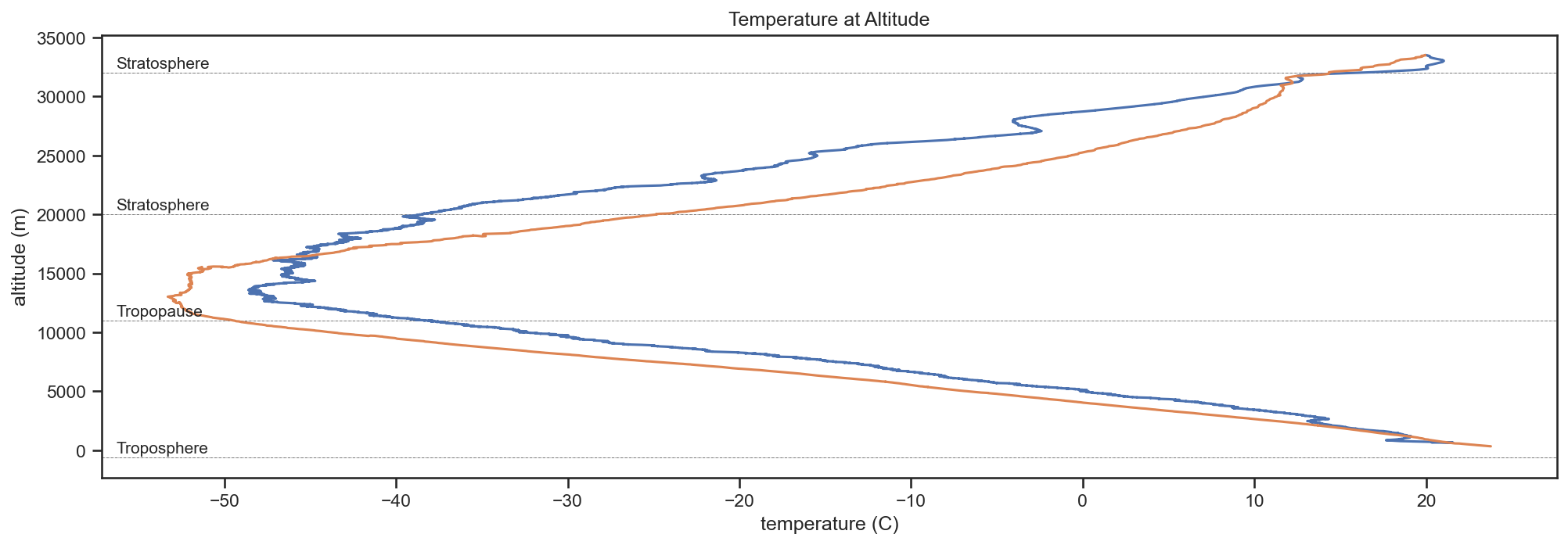
Weather Data
fig, ax = plt.subplots()

annotate_layers(ax, label=True, max_layer=4)
ax.plot(ascent_phase['temperature_C'], ascent_phase['altitude_m'], label="ascent")
ax.plot(descent_phase['temperature_C'], descent_phase['altitude_m'], label="descent");
ax.set_title("Temperature at Altitude")
ax.set_ylabel("altitude (m)")
ax.set_xlabel("temperature (C)")
Text(0.5, 0, 'temperature (C)')
# Write the missison data back out to a csv file.
mission_data.to_csv(directory + '/clean-data.csv')